
Executive summary
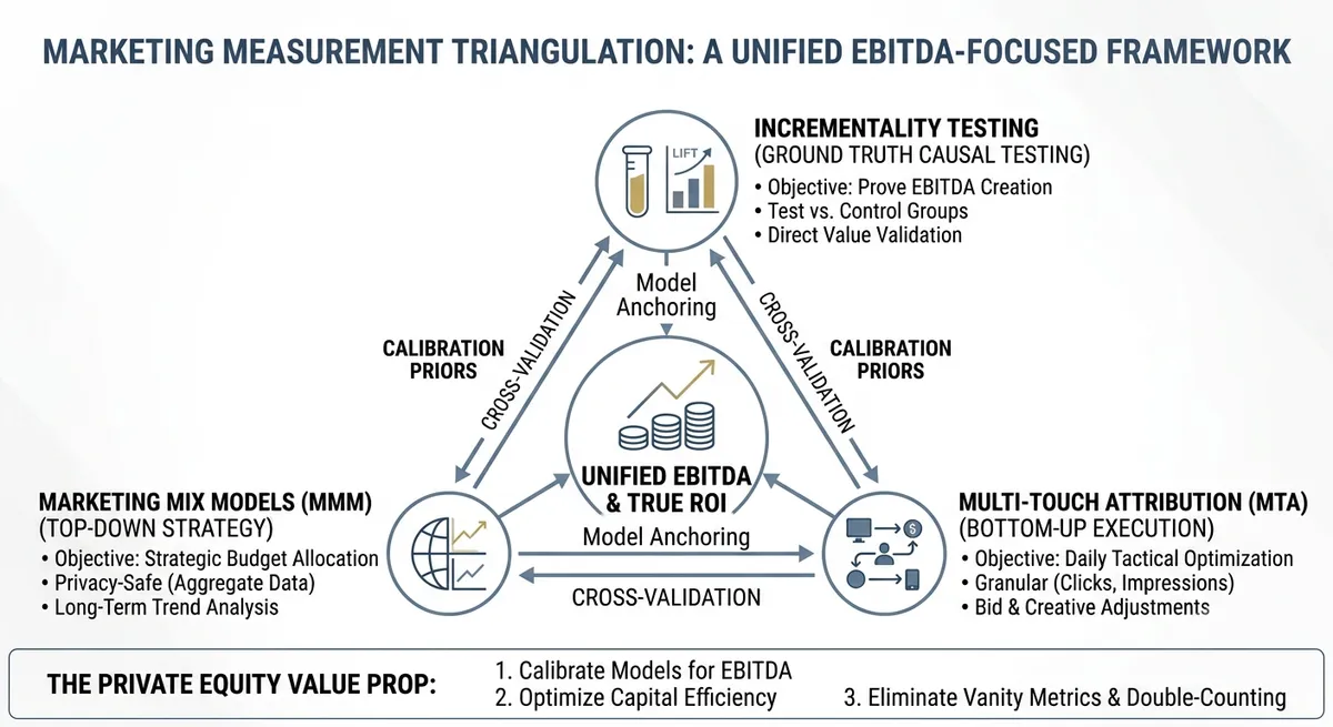
Marketing Mix Modeling and incrementality experiments answer different questions.
MMM estimates the contribution of the full marketing portfolio over time. It supports budget allocation across channels, markets, and planning horizons. Incrementality experiments estimate the causal lift of a specific intervention. They answer what happened because a campaign ran, rather than what happened while it ran.
A mature measurement program uses both. The experiment does not replace MMM. It calibrates it.
The operating question is straightforward: when a geo test produces a causal result, does it make the MMM more reliable? The answer must be measured, not assumed.
This article explains:
- how to translate experimental lift into an MMM calibration target,
- how to test whether calibration improved the model,
- what to do when experiment and MMM disagree,
- how to use both methods for budget decisions.
1) The role of each method
MMM is a portfolio model. It estimates how sales, revenue, gross profit, or contribution margin respond to media after controlling for baseline demand, seasonality, price, promotions, distribution, and other business factors.
A simplified specification is:
$$ Y_t = B_t + \sum_{m=1}^{M} g_m(A_{m,t}) + \varepsilon_t $$
Where:
- $Y_t$ is the business outcome at time $t$,
- $B_t$ is baseline demand and non-media controls,
- $A_{m,t}$ is the adstocked exposure for channel $m$,
- $g_m$ is the channel response curve,
- $\varepsilon_t$ is residual error.
An incrementality experiment estimates a treatment effect. In a geo test, that effect is usually the difference between treated and counterfactual outcomes over a defined test period:
$$ \tau = \sum_{g \in T}\sum_{t \in \mathcal{W}} \left(Y_{g,t} - \widehat{Y}^{(0)}_{g,t}\right) $$
Where:
- $T$ is the treated geo set,
- $\mathcal{W}$ is the test window,
- $Y_{g,t}$ is observed outcome,
- $\widehat{Y}^{(0)}_{g,t}$ is the counterfactual outcome without treatment,
- $\tau$ is estimated incremental lift.
The experiment gives a causal anchor. MMM gives breadth, continuity, and optimization capability.
2) Data assets, covariates, and precision
The model is only as credible as the data-generating process it can observe. A sophisticated MMM cannot recover a causal media effect when a material driver of demand is missing, poorly measured, or moves in lockstep with spend.
The most valuable data asset is not the largest table. It is a decision-grade panel: a consistent outcome, media variables with real variation, and controls for the non-media forces that changed demand. This is the foundation of both precision and causal credibility.
2.1 Start with the target, not the feature list
Choose the target that matches the decision. Revenue is acceptable when margin is stable. Where margin, fulfillment cost, returns, or promotion depth vary materially, gross profit or contribution margin is the stronger target.
The target needs to be:
- complete across the modeling horizon and geography;
- consistently defined after returns, cancellations, and accounting adjustments;
- available at the same cadence as media and controls;
- stable enough to distinguish signal from normal operating noise.
An imprecise target widens every downstream ROI interval. Better media data cannot compensate for a KPI that is revised late, inconsistently geo-mapped, or disconnected from economic value.
2.2 The minimum decision-grade data asset
For each time period and, where feasible, geography, build a governed panel with four blocks:
- Outcome: revenue, gross profit, contribution margin, or qualified demand.
- Media treatment: spend, impressions, reach, frequency, and campaign timing by channel.
- Business controls: price, promotions, distribution, inventory availability, product assortment, and sales capacity.
- External demand controls: seasonality, holidays, macro conditions, category demand, competitor activity, and local factors such as weather where economically plausible.
Granularity matters. National weekly data may be sufficient for a stable national channel. It is often too coarse for local OOH, retail media, weather-sensitive categories, or geo experiments. The useful grain is the lowest level at which the outcome, treatment, and material confounders can be joined reliably.
2.3 How to decide whether weather or another feature is needed
Do not add weather because it is available. Add it when it plausibly changes the outcome, varies independently of media, and reduces residual demand movements that would otherwise be attributed to marketing.
Use a four-part test for any candidate covariate:
- Business mechanism: Can leadership explain why the variable changes demand? Weather may matter for delivery, travel, seasonal apparel, food, utilities, or store traffic. It may be irrelevant for other categories.
- Timing and granularity: Does it align with the target’s geography and cadence? National average temperature is a weak control for a local retail outcome.
- Incremental information: Does it improve out-of-sample error, reduce residual autocorrelation, or explain known demand shocks after existing controls are included?
- Causal risk: Is it a pre-treatment driver of demand rather than a consequence of marketing or a duplicate proxy for an existing variable?
The same test applies to competitor spend, search demand, social trends, macro indicators, product launches, and inventory signals. Search volume, for example, can be useful as a demand proxy, but it can also be affected by media. Treating a post-media response as a control can absorb genuine media impact and bias ROI downward.
2.4 Covariate selection is a causal design decision
The objective is not maximum $R^2$. It is to control material confounders without controlling away the treatment effect.
For each candidate variable $X_k$, ask:
- did it affect the business outcome?
- was it correlated with media deployment or spend?
- was it measured before the marketing exposure occurred?
- can its effect be estimated separately from media with the available variation?
Only variables with a credible answer belong in the core specification. Use domain knowledge first, then test the choice with time-series and geo-level diagnostics. Automated feature selection can be useful as a challenge process, but it should not replace causal reasoning.
Collinearity is the central practical constraint. If paid search, promotions, and branded TV always move together, the model may predict total sales well while being unable to assign contribution reliably across the three. The remedy is not another algorithm. It is more independent variation: staggered launches, geo holdouts, spend changes, or experiments.
2.5 What precision means in MMM
Precision is the width of the uncertainty interval around an incremental ROI estimate, not the number of decimal places in a dashboard.
For channel $m$, define incremental ROI as:
$$ \mathrm{iROI}_m = \frac{\widehat{\Delta \mathrm{Profit}}_m}{\mathrm{Spend}_m} $$
The interval around $\mathrm{iROI}_m$ narrows when the model has:
- a cleaner and more economically aligned target;
- independent movement in channel exposure and spend;
- complete controls for major demand shocks;
- sufficient time periods, geographies, and signal-to-noise ratio;
- experimental evidence that anchors the channel effect.
It widens when media is highly collinear, the target is volatile, the business experiences unmodeled shocks, or the channel has little meaningful spend variation. A narrow interval from a misspecified model is false precision. A wider interval with transparent assumptions is more useful for capital allocation.
2.6 A practical feature-governance process
Maintain a feature register for every MMM refresh. For each covariate, record the business rationale, source, grain, transformation, availability lag, causal role, and validation evidence.
Retain a feature when it improves holdout performance or experimental agreement without creating implausible media estimates. Remove or quarantine it when it is post-treatment, poorly measured, unstable, or redundant with a better control. Revisit the register after major operating changes such as a pricing reset, new market launch, data migration, or supply disruption.
This discipline turns data assets into a compounding advantage. The model becomes more precise because the organization learns which drivers of demand are real, measurable, and decision-relevant.
3) Turn the experiment into a calibration target
Do not compare an experimental result with an MMM result informally. Put both estimates on the same basis first.
The required alignment is:
- same outcome metric: revenue, gross profit, or contribution margin;
- same treatment definition: spend, impressions, reach, or incremental exposure;
- same geographies and dates;
- same attribution window and carryover assumptions;
- same unit of analysis.
For a test of channel $m$, derive the MMM-implied lift in the test scope:
$$ \widehat{\tau}{\mathrm{MMM}} = \sum{g \in T}\sum_{t \in \mathcal{W}} \widehat{g}m(A{g,t}) $$
Then compare it with experimental lift, $\widehat{\tau}_{\mathrm{EXP}}$.
The calibration ratio is:
$$ C_m = \frac{\widehat{\tau}{\mathrm{EXP}}}{\widehat{\tau}{\mathrm{MMM}}} $$
Interpretation:
- $C_m \approx 1$: the MMM agrees with the experiment in the tested range;
- $C_m < 1$: the MMM likely overstates incremental impact;
- $C_m > 1$: the MMM may understate incremental impact.
The ratio alone is not a decision rule. It needs an uncertainty range. If the experimental confidence interval is wide, a difference from 1 may be noise rather than evidence of model bias.
4) Calibrate the model without overfitting to one test
A common failure is forcing the MMM coefficient to equal the result of one geo test. That creates a model that fits one observation and may become less reliable everywhere else.
Use the experiment as a prior or likelihood term, not as an absolute truth.
For a Bayesian MMM, encode the experimental result as an informative prior on the channel effect:
$$ \beta_m \sim \mathcal{N}\left(\widehat{\beta}{\mathrm{EXP}}, \sigma^2{\mathrm{EXP}}\right) $$
Where:
- $\widehat{\beta}_{\mathrm{EXP}}$ is the experiment-derived effect estimate,
- $\sigma^2_{\mathrm{EXP}}$ reflects experimental uncertainty,
- $\beta_m$ is the MMM channel-effect parameter.
A precise, well-executed experiment should have more influence than a noisy test. Multiple experiments should be pooled hierarchically rather than applied sequentially as isolated overrides.
For frequentist MMMs, use the result as a validation constraint. Re-estimate alternative specifications and select the model that balances:
- in-sample fit,
- out-of-sample forecast accuracy,
- plausible response curves,
- agreement with high-quality experimental evidence.
5) How to measure whether the MMM improved
A calibrated MMM has not improved because its ROI changed. It has improved only if its predictive and causal consistency improves.
Measure improvement across four dimensions.
5.1 Holdout forecast accuracy
Hold out a period, geography, or campaign that was not used to train or calibrate the model. Compare pre-calibration and post-calibration error.
Use metrics such as:
$$ \mathrm{MAPE} = \frac{1}{n}\sum_{i=1}^{n}\left|\frac{Y_i-\widehat{Y}_i}{Y_i}\right| $$
$$ \mathrm{RMSE} = \sqrt{\frac{1}{n}\sum_{i=1}^{n}(Y_i-\widehat{Y}_i)^2} $$
Forecast error should decline on unseen data. An improvement only on the calibration window is not proof of a better model.
5.2 Experimental agreement
For each eligible experiment, compare the observed lift with the model-implied lift before and after calibration.
A useful score is weighted experimental error:
$$ \mathrm{WEE} = \frac{\sum_{j=1}^{J} w_j\left|\widehat{\tau}{\mathrm{MMM},j}-\widehat{\tau}{\mathrm{EXP},j}\right|}{\sum_{j=1}^{J}w_j} $$
Weights $w_j$ should reflect experimental precision, relevance, and execution quality. A large, clean experiment should count more than a small or contaminated one.
The post-calibration model should reduce WEE on experiments that were not used in calibration.
5.3 Parameter stability and plausibility
A better model should not require unstable channel effects.
Check whether calibration causes:
- large swings in channel ROI between model refreshes;
- implausible adstock half-lives;
- response curves with no saturation or excessive saturation;
- sign reversals without a business explanation;
- an unexplained shift from media contribution into baseline demand.
If a model achieves a lower error by producing implausible economics, it has not improved. It has become overfit.
5.4 Decision stability
The final test is decision quality.
Run the budget optimizer before and after calibration. Assess whether the recommended allocation is:
- directionally consistent with validated experiments;
- stable under reasonable parameter variation;
- feasible within channel, market, and operational constraints;
- expected to improve marginal return rather than only average ROI.
A model that changes the annual media plan by 40% because of one small test is a governance problem, not an insight.
6) What to do when MMM and incrementality disagree
Disagreement is useful. It shows where the measurement system needs investigation.
Do not immediately declare either method wrong. Start with a structured diagnostic.
6.1 Check the experiment first
Review:
- treatment and control balance before launch;
- parallel trends in the pretest period;
- power and minimum detectable effect;
- media leakage into control geographies;
- changes in price, promotions, inventory, or distribution;
- outcome-data completeness and reporting lag;
- the counterfactual model and its residuals.
A weak experiment should not recalibrate a portfolio model.
6.2 Check the MMM specification
Review:
- spend and exposure data quality;
- channel collinearity and concurrent campaigns;
- adstock and saturation assumptions;
- control-variable coverage;
- treatment of promotions, holidays, supply constraints, and competitors;
- priors and parameter bounds;
- residual autocorrelation and structural breaks.
MMM often overstates a channel when spend is correlated with latent demand. It can understate a channel when a campaign has long carryover that is not captured in the model.
6.3 Choose the right response
There are four common outcomes:
- Experiment is clean; MMM is inconsistent. Recalibrate the channel prior or re-specify the response curve.
- MMM is stable; experiment is weak. Treat the test as directional evidence and rerun it with better power or controls.
- Both are credible but operate in different conditions. Segment the model by market maturity, audience, product, or spend range.
- Both are noisy. Do not force a budget decision. Improve data quality and commission another test.
The objective is not to eliminate disagreement. It is to explain it and reduce it where it affects capital allocation.
7) The operating model: an experiment-to-MMM loop
Triangulation works when it is an operating rhythm, not an annual modeling project.
A practical cadence is:
- use MMM to identify channels with high budget, high uncertainty, or suspected saturation;
- prioritize those channels for incrementality testing;
- run geo tests with pre-registered hypotheses and quality gates;
- convert validated lift into calibration evidence;
- re-estimate the MMM and backtest it;
- update budget scenarios and decision thresholds;
- record the evidence, assumptions, and remaining uncertainty.
This loop turns experiments into a learning portfolio. The next test is selected because it has the highest expected value of information, not because it is the easiest campaign to isolate.
8) Executive scorecard
A leadership team does not need every model diagnostic. It needs a compact view of whether the measurement system can support investment decisions.
Track:
- percentage of spend covered by validated MMM response curves;
- percentage of high-spend channels calibrated against incrementality evidence;
- out-of-sample forecast error before and after calibration;
- experimental agreement on holdout tests;
- confidence interval for incremental ROI by channel;
- budget reallocated because of validated evidence;
- realized return versus the approved investment case.
This is the bridge between data science and capital discipline.
Closing
MMM is strongest when it is challenged by experiments. Experiments are strongest when their evidence is scaled through MMM.
The gold standard is a closed-loop system: MMM identifies where uncertainty is expensive; incrementality tests establish causal anchors; calibration improves the model; and the model reallocates capital with more confidence.
That is how measurement moves from reporting past performance to managing future return.
Selected references
Google describes modern measurement as combining methods that “capitalise on their strengths and complement their weaknesses.” That is the practical case for triangulating attribution, experimentation, and MMM rather than relying on one source of evidence.
- Google: The modern measurement playbook for its framework linking attribution, MMM, and incrementality.
- Google Meridian for an open-source Bayesian MMM framework and its model documentation.
- Lewis, R. A., and Rao, J. M. (2015). The Unfavorable Economics of Measuring the Returns to Advertising. The Quarterly Journal of Economics. A useful reminder that advertising-effect estimates can be statistically noisy even with large datasets.
- Angrist, J. D., and Pischke, J.-S. (2009). Mostly Harmless Econometrics. The reference text for thinking clearly about identification, controls, and causal inference.
- Farris, P. W., Bendle, N. T., Pfeifer, P. E., and Reibstein, D. J. (2020). Marketing Metrics. A practical reference for linking marketing measurement to financial outcomes and operating decisions.
- McKinsey Global Private Markets Report for the broader private-capital context in which evidence-backed value-creation plans are assessed.